Written By Aaron Spaulding

This week I updated the classification model from the baseline result. I tested multiple configurations changing the transfer learning approach, augmentations applied, and classification model architecture. Since I have many results I include just the worst and best performers.

Worst Model

This model was by far the worst performer with almost no predictive ability. The plot of accuracy vs. epochs shows how the model was unable to converge for either the test or train sets, never passing 20% accuracy.

The confusion table reveals more into this and shows how the model only predicts one type of bird, the cardinal.

Best Model

The best model I developed was developed using the “resnet_v2_152” as a base model with three dense layers for the classification model. The first two had sizes 64 and 32 with the ‘relu’ activation function and the final layer had size 19 (19 classes) with the ‘sigmoid’ function. For this, I used a learning rate of 0.001. My early stopping stopped training at 33 epochs after the model converged. To double-check I trained the model for 10 additional epochs however the model did not improve from before. The image below shows the model loss vs. epochs and may indicate some overfitting occurring. I also applied all the discussed augmentations and balances the train and test sets.

The confusion table also is much improved with many more predictions along the diagonal.

This model was able to achieve a final micro-F1 of 63.54. This is a fantastic result since this score on a recent bird classification challenge on Kaggle would be a top 2% submission.

Written By Aaron Spaulding

This week I received the initial results of our classification method. Most of the time this week was spent writing the code for the method and setting everything up to run properly. However, I was able to set a baseline result which we can improve on in the upcoming weeks!

Baseline Result

It is important to note that this is a baseline result. This means we use a simple model without applying augmentations or optimizations. This also means our next models should be improvements from this!

This baseline model was built with the “resnet_v2_152” as the base model for transfer learning. I used three dense layers as my classification model and saved 25% of the dataset for validation.

The figures below show the loss and accuracy as the model is trained. The model quickly overfits the training set and stops learning on the test set. This leaves us with accuracy just below 60%.

To also test performance I created a confusion table for all our species. It is clear that the model is not a strong performer. In addition, we can see that the classes are not balanced which may be contributing to the low accuracy score.

Written By Aaron Spaulding

During the past week, I continued working on the classification model that will be used to determine the species of a bird sound after detection. Most of the week was spent processing the clips we labeled over break and applying augmentations. The image below shows the process I created where I import the audio data for each clip, mix it with Gaussian noise, and then generate a spectrogram with 251×251 shape. These processed clips will be used to train and validate our initial classification models.

One example of this process is shown below for the northern cardinal (Cardinalis cardinalis). The first image shows a picture of the bird taken this winter and the second shows the fully processed spectrogram ready for training.

This week I also met with Paul to record the 24-hour dataset. We set the arrays and temperature sensor up to record in my yard. We were able to capture the full 24-hour dataset with birds and temperature!

Written By Aaron Spaulding

During the past week, I started the classification model that will be used to determine the species of a bird sound after detection. Since this is an entirely new model a lot of time was spent reading literature and reviewing other work on this topic.

After discussion with the sponsor an outline for our method has been finalized. Some of the things we will try are augmentations, using transfer learning, and training on spectrograms instead of audio clips.

Augmentations will be useful since we have a limited dataset. I plan to apply the following after separating my train/test sets to help expand the data.

• Time shifts
• Time reversal
• Time scaling
• Vertical frequency shifts

Combinations of these with different values will be applied to artificially expand the data and could help the models.

I also plan to also use transfer learning. I found three models that may perform well. These include the VGG-19, Resnet V2, and EfficientNet models. Each of these has been pretrained on ImageNet, a collection of images with 1,000 classes, and may generate relevant features. The image below shows the VGG-19 architecture.

The final step will be to train our classifier model on top of the features generated by the pretrained model. For this, we will test a linear model and a simple neural net.

Written By Aaron Spaulding

During the past week, I focused on adjusting the plane-wave simulation scripts to work on our multichannel arrays. This week I also wrote codes to extract metrics the sponsor defined. A list of these is shown in the image below.

The images below show the raw beampattern and labeled beampattern marked at the beam-width locations.

Written By Aaron Spaulding

During the past week, I focused on developing the scripts to plane waves incident on the array. By calculating the time offsets of a single tone I was able to create synthetic multichannel audio clips. The images below show the beamformer beam pattern outputs as a source rotates around the 4-channel array. These were calculated on the outputs of my script.

This will be used in the next steps of beamformer validation where we will measure the beam responses, and sponsor defined metrics for our array and beamforming method!

Written By Aaron Spaulding

During the past week, I explored other possible ensembling methods as we expand our model. I tested three methods, fitting a ridge regression, a linear model, and taking an average of the three models used last week. I limited the ensembling methods to more simple regression methods to help reduce overfitting that could develop when using larger models with more parameters.

Linear Ensemble

The first new method I tested was fitting a linear model to the model outputs. While this method should produce results close to the mean, actual performance with an AUC of 78.18 showed a decrease in predictive ability. An AUC of 78.18 is lower than each of the individual models.

Tikhonov Regularization (Ridge Regression)

I also tested Ridge Regression to see if ensemble performance could be improved with a more general solution. This method produced a slightly better result but still suffered for many of the cases with an AUC of 78.16.

Average Ensemble

This third method is the most simple and should not underperform any individual model. The average ensemble performs the strongest with an AUC of 86.28.

Written By Aaron Spaulding

During the past two weeks, I focused on building the classification model and further expanding the current detection method.

Classification Method

The first step in developing our classification method is to construct our synthetic dataset of bird sounds native to our region. Last week I started writing the code to combine labeled bird sounds with our noise sources. The next step will be to run this with noise sounds captured by the array.

The Ensemble

This week I also expanded the detection model. Our current efforts have focussed on developing a single well-performing model, however building and testing an ensemble could improve overall performance. To test this I constructed an ensemble composed of three models, the GBM, RF, and the BART. Each of these was evaluated with a 4-fold random CV on the BirdVox-DCASE-20k dataset to help improve training speeds.

GBM

The GBM is the model currently in use by our detection method. This model achieved an AUC of 86.29 (the slight drop in performance is due to the low number of folds in the cross-validation) and had a good separation of variables.

RF

The random forest often performs similarly to the GBM when tuned. I used the ranger package on R with a default value of 500 trees and using Gini impurity to measure variable importance. This model performed similarly to the GBM with an AUC of 85.88. This may improve after tuning parameters (the GBM AUC increased almost by 1 point after parameter tuning and with a 100-fold CV. A similar increase would make this model out-perform the current GBM.) The image below shows the CDF of model predictions.

BART

A bayesian additive regression tree model was also built and measured. This model was built with 150 trees using the R BART package. This model performed the lowest by AUC standards at 84.74, however, this model also leaves the most room for improvement and could be tuned.

The Average Ensemble

Combing these models by averaging outputs produced a result better than the RF or BART individually but slightly worse than the GBM with an AUC of 86.28. This result shows that if the RF or BART models were tuned ensemble performance could be greater than just using the GBM. The image below shows the distribution of results for the combined model.

Future Work

The next steps on the ensemble should include tuning the BART and RF models. It may also be beneficial to compute optimized weighted averages for the ensemble as well as possibly building a GLM or linear model to combine the output.

Written By Aaron Spaulding

Variable Analysis

During the past semester and over the holiday I designed new features efforts to improve the detection model. While the detection model is now great, we now have over 240 predictors in our dataset which is not ideal and could lead to overfitting. This should also be addressed since we may need to design new predictors when building the classification model.

Variable Importance

I previously used relative variable importance when developing new features. Over the break, I removed a low weighted set of features, the frequency percentiles, and was able to slightly improve model performance. Figure 1 shows the variables with the highest relative importance to the GBM.

The “s_energy_band” feature set has almost half the relative importance. I designed the “energy_band” features to quantify the energy of normed bands of the spectrogram, an aspect that could be helpful when analyzing audio clips. Figure 2 shows the lowest and highest frequencies of the highest weighted bands.

A couple of conclusions could be possible.

• Bird calls commonly occur inside these frequency bands.
• Not bird calls such as noise or predators occur commonly insides these bands.

PCA

Principle component analysis (PCA) is another method used when analyzing variables. Using 240+ variables is possible when the dataset is large but is not possible when data is scarce. Reducing the number of dimensions can also decrease model training time and may provide insight into correlated variables.

Running PCA revealed that 90% of dataset variability could be contained in just 10 principal components. This also revealed a high correlation in the frequency percentile set. One surprising result was the correlation between some energy bands and some Spectral components, something we will have to discuss and investigate in the future.

Running the models on just principle components did reduce performance with K-Fold CV, bringing AUC to 81.00. This is expected however and could be improved by including more principle components in the model.

Written By Aaron Spaulding

BirdVox-DCASE-20k Parameter File

This week I wrote the codes to build the parameter file for the BirdVox-DCASE-20k dataset. This parameter file includes each feature for each audio clip and will be used to train and test our initial models. Each feature was calculated after processing each audio clip with our bandpass filter and our pre-emphasis filter. On my laptop, each audio file took about a second of processing time and total runtime was a little more than 6 hours.

Variable Importance

Measuring variable importance can give valuable insight into how the model works and what features contribute the most to solving the bird-detection problem. Figure 1 shows the 18 highest weighted features of a GBM trained on 90% of the BirdVox-DCASE-20k dataset.

It is interesting that the model “likes” spectral features and does not heavily rely on frequency percentiles. (We expected otherwise.) It is possible the frequency percentile and frequency at the highest energy point features do not work well in extremely noisy environments and maybe steps will need to be taken to help reduce noise even further. It may be beneficial to use Mel-frequency spectral-based features since other spectral features have heavy weightings.

Detection Model

This week I also built the first detection model. This was run with 4-fold cross-validation to obtain predictions on the entire BirdVox-DCASE-20k dataset. Average NASH and RMSLE (0.21 and 0.31) both scored well across all four-folds and overall model performance was great for a baseline model with an AUC 79.37. (This model is untuned and has not been optimized.) This is a good baseline since similar models on similar data were able to achieve an AUC between 80 and 90 and none in “The first Bird Audio Detection challenge” [1] were able to get over 90 AUC.

Figure 2 shows a CDF of model predictions and is exactly what we would expect. Figure 3 shows the number of false positives and false negatives as functions of potential threshold values and represents decent, but not great, performance.

In order to more accurately visualize the model performance, I plotted the predicted class probabilities for each class. This clearly shows the separation of variables and clear separate peaks for the bird cases and nonbird cases

To see the model performance in greater detail I also plotted the normed predicted class probabilities of the predictions. A good model would have clear peaks and very little overlap in each region. While distinct peaks are visible the model does struggle on a number of bird calls and incorrectly identifies a large portion of the bird calls as having no bird call.

Next Steps

Next steps will include revisiting the beamforming algorithm to fix the errors in the FIR FD filter and to examine some of the cases that the model struggles on to help improve performance.

[1] Stowell, D., Stylianou, Y., Wood, M., et al.: Automatic acoustic detection of birds through deep learning: the first bird audio detection challenge. Methods Ecol. Evol. 10, 368–380 (2018)

Written By Aaron Spaulding

Pre-Emphasis Filter

This week I wrote the code for our pre-emphasis filter. This filter is represented by the function in Figure 1 and has been shown to be helpful in many speech detection algorithms. The team is currently using an alpha value of 0.95. This may be changed in the future after some tuning.

The attached plots show the difference between raw audio captured by the team and the same raw audio after being processed by the pre-emphasis filter. While the difference is not dramatic in the time domain signal, the frequency domain signal is almost completely transformed.

Feature Analysis

This week I also wrote codes to extract and analyze some of the features in our feature set.

Frequency Percentiles

This group of features is built by generating a CDF of the highest energy frequency in successive windows and then sampling this CDF. These sampled values are plotted on a spectrogram and show how some of these are able to “line up” with the bird calls.

Frequency at Highest Energy Points

This group of features is built by taking the highest energy frequencies at the highest n energy windows of the signal. This produces similar but slightly different results compared to the frequency percentiles and these are also shown plotted on the same signal.

Written By Aaron Spaulding

The Beamformer

Over the past two weeks, I was able to build the time-domain and frequency-domain beamformers for the project. Neither of these are precise enough or fast enough for our project. (The time-domain beamformer has limited accuracy since time-delays must be integer multiples of the sampling rate while the frequency-domain beamformer must take the FFT of the entire sequence leading to very slow calculation times for long sequences.)

The goal of this week was to create a Fractional Delay(FD) FIR filter to implement the time shifts. A successful beamformer using this method should be able to run nearly as fast as the time-domain beamformer with similar precision to the frequency-domain beamformer.

I was able to build the fractional delay FIR filter following a chapter in a text-book I found here. To help reduce the size of the filter needed a time-domain shift is used to reduce the required FIR shift to less than 1. This means it should be possible to build a FIR filter of size 3 that meets all our requirements.

The results were not ideal and the beam-pattern created with this method does not reflect our expectations. The artifacts introduced are probably due to the design of the FIR filter which needs refinement.

The Bandpass Filter

Previously I had written a bandpass filter using a boxcar window. This method is not ideal as severe artifacts are introduced when using this method. I wrote the code for three other filters to fix these issues.

Butterworth and Chebyshev Filters

The first filters I built were the Butterworth and Chebyshev filters. These work well and give frequency response results that seem optimal, but are still not ideal since group delay is not zero.

FIR Filter

To fix the group delay problem I designed a FIR filter for the bandpass filter. This FIR filter should have close to zero group delay and also should have a good frequency response. In addition using this method lets us implement the bandpass filter with a convolution which is a very inexpensive operation leading to a quick filter.

Written By Aaron Spaulding

The Beamformer

This week I expanded on the beamformer code and fixed some of the issues present in the time-domain implementation I wrote last week. One limitation of the Delay-And-Sum (DAS) beamformer in the time domain is that shifts may only be performed in integer multiples of the sampling rate — introducing errors in the results and limiting the resolution of the beam pattern.

One solution I programmed this week implemented the delays in the frequency domain. The algorithm takes the FFT of the time domain signal, applies a phase shift, (a phase shift in the frequency domain is the same as a delay in the time domain) sums the signals, and then takes the IFFT to create the beam projected in a given direction. This method allows for shifts smaller than the sampling rate. The images below were both created with the same angles, same array, and same synthetic audio. These beam responses illustrate the dramatic improvement when implementing the DAS beamformer in the frequency domain.

The Array

This week I also created beam patterns from samples captured by the Array. (Using audio captured by Paul.) These results show that our functions work correctly and are able to accurately detect the angle of the sound source. The image below shows a beam response in response to a bird sound played from a Bluetooth speaker five feet from the array at an angle of zero degrees. The response shows how the array is able to accurately “point” towards the sound and is able to pick up a synthetic bird sound.

Written by Aaron Spaulding

This week I wrote and tested parts of the beamforming code. Since our hardware has not been finalized the code was all written to be independent of array structure. This means all offsets and other values that depend on the array are calculated as the array is defined. This should limit code refactoring if we switch to a three-dimensional array. As usual the code is published on the GitHub here.

The Array

The distance of each microphone to a plane wavefront incident on the origin must be calculated. This must be known for every microphone and every beamforming angle. Since the array might change we must be able to define a method to automatically calculate these offsets. Figure 1 shows a diagram I created that depicts this scenario for one microphone.

The problem could be simplified by placing the plane wavefront on one of the microphones. This simplifies some calculations since one microphone has no time-shift; however drawing the diagram this way lets us place microphones anywhere and still calculate distances easily. Figure 2 shows the equations for this method for a two-dimensional array.

This may be expanded to a three-dimensional array by adjusting the angle definition.

The Beamformer

This week I also wrote the code for the beamformer. This code implements a Delay-And-Sum(DAS) beamformer in the time-domain. This imports the audio channels, offsets each channel by the set of time shifts for each beam, and outputs the single-channel audio for each beam. Figure 3 shows this process.

This was run on a test sample where a plane wave was simulated for a linear five-channel array. A plane-wave superimposed on noise was simulated for each microphone. Beams in 360 directions were then calculated. The image below shows the energy level of the beam by beam direction. A peak clearly “points” in the direction of the plane wave source and is mirrored over the line-array.

Next week I hope to implement the DAS beamformer in the frequency domain. This should be more accurate than the time-shift method since shifts would not have to occur in integer multiples of the sampling rate.

Written by Aaron Spaulding

Feature Extraction

This week we decided on a list of features and split up the task of writing the feature extraction codes. Table 1 shows features I defined and wrote code for this week.

Image 1 and 2 show CDF’s created by this method where dashed red lines show the sample locations. These were created from random inputs from the “BirdVox-DCASE-20k” dataset. (Clips “000db435-a40f-4ad9-a74e-d1af284d2c44.wav” and “00053d90-e4b9-4045-a2f1-f39efc90cfa9.wav”

“Better Than MFCC Audio Classification Features” (G. Ruben (2013))

The second set of features were included in “cepstralSpectral.py.” These include power, energy, spectral centroid, bandwidth, and zero_crossing_rate. (The zero_crossing_rate represents the number of times the time-series signal crosses the x-axis.) This code also defines the first fifteen spectral and cepstral coefficients as defined here. (G. Ruben (2013)) We extract the first fifteen from each analysis since we do not have any major computational limits. These coefficients represent a set of features that may include principal components and are detailed more in the paper.

Other Code

A large portion of the week was also spent writing supporting code for the feature extraction and for handling large amounts of data. I wrote a wrapper for the “pydub” python library and defined my own Audio object that contains the pre-processed time-series and Fourier series data that we will need. The import code I wrote also supports multithreading, which is new and should allow for faster imports when dealing with our larger datasets.

In addition to these functions, I also defined helper functions to make analysis easier. I also a wrote a python filter function, as well as functions to plot and export graphs and spectrograms. These all also support multithreading as well.

Beamforming

I also made some progress with the beamforming algorithm. I was able to finalize some of the code for the linear array which now does work.

---

Y. Tseng (2020) Yi-Chin Tseng, Bianca N. I. Eskelson, Kathy Martin & Valerie LeMay (2020) Automatic bird sound detection: logistic regression based acoustic occupancy model, Bioacoustics, DOI: 10.1080/09524622.2020.1730241

G. Ruben (2013) Gonzalez, Ruben (2013/10/01) Better Than MFCC Audio Classification Features, 10.1007/978-1-4614-3501-3_24 https://core.ac.uk/download/pdf/143870996.pdf

Written by Aaron Spaulding

Beamforming

During the last week, I wrote the beamforming code for a linear microphone array. I tested two methods; the first using time-shifts in the time domain, and the second using complex demodulation in the frequency domain. The design of these algorithms was based on slides presented by the sponsor. These methods are published on GitHub and were presented to the sponsor and the team.

Machine Learning Models

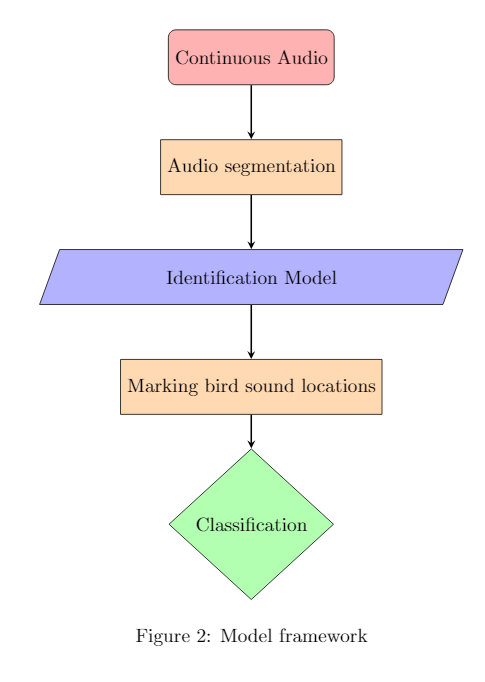
This week I proposed a model framework. The overall model framework is shown in Figure 2 which depicts the separation of identification and classification steps. This should result in faster performance and may help result in faster, smaller, and easier to understand models.

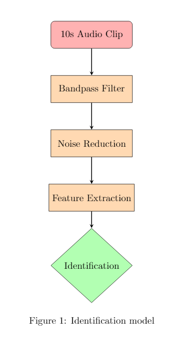
Figure 1 shows the outline of the identification model I proposed. I suggested using a model ensemble consisting of the GBM, RF, BART, and GMM models. This combination should allow for clear analysis of input variables and may provide good results. Other papers had success using just an RF(Random Forest) model. (Plumbley et al. (2014)) The addition of the GBM, BART, and GMM models has, to my knowledge, not been done for this problem before.

I compiled a list of possible features that could be used for the identification model. Feature extraction is an important step that may affect the model more than even the model parameters.

Datasets

These machine learning models do not require nearly as much data as similar deep learning models. Using small datasets may not dramatically decrease model performance for bird sounds. (Oliveira et al. (2020))

I proposed using two datasets. The first “BirdVox-DCASE-20k”(Lostanlen et al. (2018)) is compiled in part by Cornell Lab of Ornithology and contains twenty-thousand labeled ten-second audio clips. The second is a synthetic dataset created by overlaying open-source bird sounds from xeno-canto on noise recordings. (Tseng et al. (2020)) Using noise samples captured by the array may also help remove bias that may occur when applying the machine learning models to audio captured by the array.

I wrote the code to search for and download xeno-canto audio files by bird and quality. I also wrote the code that combines bird sounds with synthetic or recorded noise. This code can be used to create the synthetic dataset and is also published on the GitHub.

---